The rasterization pipeline

There are many ways to generate images. If we ignore ray tracing for now, the mainstream consumer graphics APIs — OpenGL, OpenGL ES, DirectX, Vulkan, and Metal — have settled on an approach called rasterization. There are plenty of good books that explain the rasterization pipeline, so I won’t go into too much detail here. Instead, I want to summarize it to introduce essential terminology.

Rasterization-based renderers approximate the surface shape of objects in the scene using simple geometric primitives, most commonly triangles. Primitives are defined by vertices that represent their location in space; for example, a triangle requires three vertices to represent its three corners.

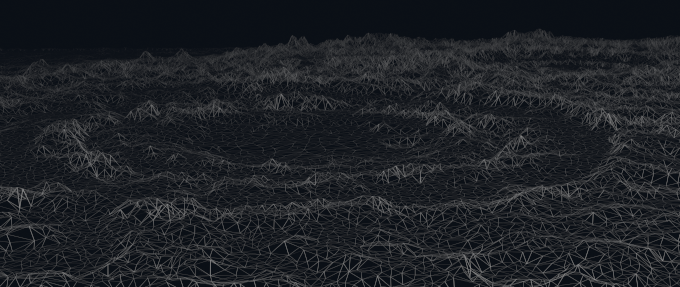
Vertices provided by the application are defined in an object-local coordinate system. Per-vertex processing must transform them into the correct on-screen coordinates, and compute any additional vertex data payload that is required.

Images are rendered by converting the vector form of each triangle into discrete pieces, called fragments, that can be colored in. This process of converting a vector triangle into fragments is called rasterization. Each pixel in the framebuffer contains one or more discrete sample points. Rasterization tests which of these sample points are inside the current primitive, and covered sample points will trigger fragment shading.

Each fragment shader invocation produces the result for a single fragment. Fragments are commonly pixel-sized but can be smaller when using sample-rate shading on a multi-sampled framebuffer, or larger when using variable-rate shading to reduce shading frequency. Fragment results can be used for one sample or can be shared by multiple sample points.

The surface color of the object is computed for each fragment and stored at the appropriate sample coordinate in the output framebuffer. Fragment colors may be transparent, which requires blending the fragment’s color with the existing color stored at its location by earlier rendering.

Determining visibility

One of the big challenges faced by graphics APIs is determining which parts of which objects are visible in the final image.

Traditional software rendering uses the painter’s algorithm. Objects must be rendered from farthest to closest. The last one drawn at a location is the one that users see, just like an artist painting on canvas. This requires the application software to ensure perfect depth sorting of all primitives. This can work for lightweight games, but is prohibitively expensive for modern content that offloads high-complexity vertex animation to the GPU.

The approach that rasterization APIs use is a per-sample depth test. A depth image is created alongside the color image, storing the distance between the currently rendered surface and the camera for each sample location in the framebuffer. When a new fragment is rendered, its distance can be compared against the distance of the already-rendered sample stored at that location. If the new fragment is closer, its color value is stored and the depth is updated. Otherwise, it is discarded because it would be behind the fragment that has already been rendered.

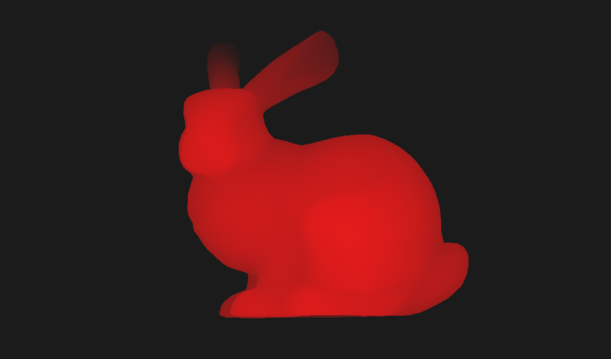
This removes the need for perfect sorting of opaque primitives. Primitives can be sent in any order, and only the parts that are closest to the camera will be visible in the final image.

Rendering of translucent surfaces, such as colored glass, requires blending the surface color with the color of the objects behind it. Most algorithms still depend on accurate sorting of translucent layers, starting rendering with the primitives farthest from the camera first, then working closer.

Rasterization pipeline

The behavior of the rasterization APIs is defined as a sequential set of stages that process the data, more commonly known as a processing pipeline. Users provide the data inputs at the start of the pipeline. Each stage generates data that flows to the next stage, and the user-visible result is produced at the end.

Minimal data sharing

Pipelining is an approach that can keep multiple hardware units busy by allowing different pieces of work to be concurrently active in different pipeline stages. This concurrent work can come from the same batch submission, such as a render pass or a draw call, or from different submissions. However, concurrently processing multiple pieces of work is only possible if there is no data dependency between them.

Graphics APIs are designed with limited data sharing across individual pieces within a batch. This removes the need for most synchronization, allowing GPU hardware to exploit the parallelism inherent in the pipeline to improve performance and efficiency. Lack of data dependencies also makes it easier to make pipeline stages wider, processing more work in parallel for higher throughput.

Thick API abstraction

Common CPU abstractions, such as C and C++, are very thin. Almost every action a program takes is visible to the wider program, with strict rules to ensure consistency of memory values observed by different threads. This means CPU hardware designs from multiple vendors often look similar when targeting similar performance levels. They are constrained by the requirements of the programming languages and their memory models.

Conversely, the high-level GPU APIs are specified so that applications can only observe the output after an entire batch submission exits the GPU pipeline. The thick abstraction used by the APIs, combined with the more restrictive data sharing within batches, gives GPU hardware designs a lot more flexibility.

GPU designs can restructure and reorder the pipeline’s internal scheduling, which is allowed as long as the correct values are produced at the end of the pipeline. GPU designs can vary which intermediate values are produced, when they are produced, and whether they are stored to memory. The user does not need to be aware of these internal choices. As a result, GPU designs from different vendors are much more varied than contemporary CPU designs.

Vendor design variation is functionally transparent to the application developer, as all designs must meet the requirements of the API specification. However, design variation is often visible as performance side effects. You can optimize your application by factoring in the behavior of the GPU you are running on. Many of the topics covered in this book fall into this class of optimization.