 |
OpenGL ES SDK for Android
ARM Developer Center
|
|
OpenGL ES SDK for Android
ARM Developer Center
|
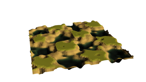
This sample uses OpenGL ES 3.1 and the Android extension pack to procedurally generate complex geometry in real-time with geometry shaders.
The Android extension pack adds many new features to the mobile platform. Some features have been exclusive to desktop OpenGL for a long time, such as geometry and tessellation shader stages. In this sample, we showcase the use of geometry shaders to generate meshes from procedural surfaces, in real-time.
The source for this sample can be found in the folder of the SDK.
The geometry shader is an optional programmable stage in the pipeline, that allows the programmer to create new geometry on the fly, using the output of the vertex shader as input. For example, we could invoke the geometry shader with a set of N points using a single draw call,
and output a triangle for each such point in the geometry shader,
In this demo, we use geometry shaders to output a variable number of triangles (up to 6), given a set of points in a grid as input. For a more in in-depth introduction to geometry shaders, see [6].
In traditional 3D graphics, we are used to thinking about surfaces as a set of connected triangles. Modelling such surfaces involve meticulous placing of points, and connecting them together to make faces. For certain types of geometry, this works alright. But making natural-looking, organic geometry is a very tedious process in this representation.
In this demo, we will take advantage of recent advances in GPU hardware and use a more suitable surface representation, to generate complex surfaces in real-time. Instead of describing our surface as a set of triangles, we will define our surface as the set of points where a function of three spatial coordinates evaluates to zero. In mathematical terminology, this set is known as the isosurface of the function, and the function is referred to as a potential.
It might be difficult to imagine what that would look like, but think of it like this: An elevation map can be considered as a function, which takes a point (x, y) in the plane and gives the height at that point. The set of points where the height is equal to a specific value is called an isoline, because it traces out a curve in the plane. An isosurface is the same concept, but bumped up one dimension.
Isosurfaces are nothing new. They have been commonly used to visualize simulations in computational fluid dynamics, or in medical imaging to visualize regions of a particular density in a three-dimensional CT scan.
I've criticized triangles as being unfit for modelling organic geometry, so I better prove to you that this isosurface stuff is somehow better! To that end, let's take a look at how you might make some simple terrain.
Let's begin with a plane. For that we need a function which is negative below the plane and positive above it. When a point is on the plane, the function is zero.
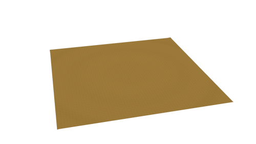
In code this could be described as
surface = p.y;
where p is the sampling point in 3D space, and surface is the function value as stored in the 3D texture. Terrain usually has some valleys, so let's add a value that oscillates as the sampling point travels the xz-plane.
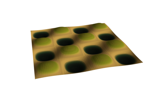
surface = p.y;
surface += 0.1 * sin(p.x * 2.0 * pi) * sin(p.z * 2.0 * pi);
Getting there, but this hardly looks like something you would find in nature. A common tool in procedural modelling is to use noise. There are many varieties of noise, such as simplex-, Perlin- or Worley-noise ([8], [9], [10]), that can be used to make interesting perturbations.
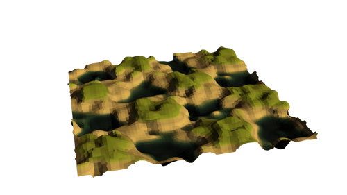
surface = p.y;
surface += 0.1 * sin(p.x * 2.0 * pi) * sin(p.z * 2.0 * pi);
surface += 0.075 * snoise(p * 4.0);
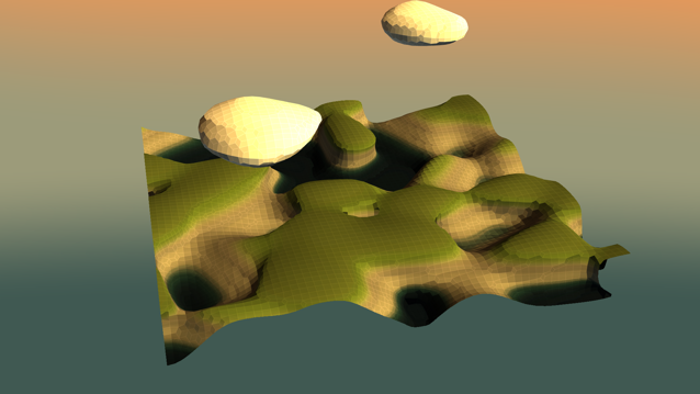
This is pretty good. But let's say we want the terrain to flatten out at the top. To do this, we can intersect the surface with a plane that is facing downwards and cutting the terrain through the tops.
surface = p.y;
surface += 0.1 * sin(p.x * 2.0 * pi) * sin(p.z * 2.0 * pi);
surface += 0.075 * snoise(p * 4.0);
surface = max(surface, -(p.y - 0.05));
We encourage the reader to have a look at Inigo Quilez's introduction to modelling with distance functions [5]. Our demo doesn't rely on the potential function being a distance field - that is, the value describes the distance to the closest surface - but the article describes some mathematical tricks that still apply. Nevertheless, this short exercise should have shown how compact we can represent the geometry, and how the representation allows for much easier experimentation, than a conventional triangle description.
Now that we have a sense of what isosurfaces are, and how we can make them, we need a way of drawing them. There are many methods for visualizing isosurfaces; some based on raytracing, some based on generating a polygonal mesh. We do not intend to give an overview of them here.
A famous method in the latter category is the marching cubes algorithm. Its popularity is perhaps best attributed to the splendid exposition by Paul Bourke [4], which does a fine job at explaining the technique, and provides a small and fast implementation as well.
In the demo, we use a different meshing technique known as surface nets. This technique appears to give similar mesh quality as marching cubes, but with considerably less geometry. Less geometry means less bandwidth, which is important to keep your mobile GPU happy.
The marching cubes technique was initially published in 1987, and is getting rather old. Not surprisingly, a lot of research has been done on the subject since then, and new techniques have emerged. Surface nets is a technique that was first introduced by Sarah Frisken [1] in 1999. The large time gap between the two techniques might lead you to believe that there may be a similar gap in complexity. But surprisingly enough, the naive version of surface nets [7] is simple enough, that you may even have thought of it yourself! Let's first take a look at how it works in 2D.
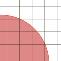
We begin by laying a grid over the surface domain. In every cell of the grid, we sample its four corners to obtain four values of the potential function. If all values have the same sign, then the cell is either completely inside or outside the surface. But if there is a sign change between two corners, then the function must have intersected the edge between them.
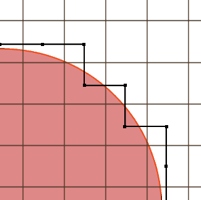
If we place a single vertex in the center of each cell that contains an intersected edge, and connect neighbouring cells together, then we get a very rough approximation of the surface. The next step is to somehow smooth out the result. In the original paper, Gibson proposes an iterative relaxation scheme that minimizes a measure of the global surface "roughness". In each pass of this routine all vertices are perturbed closer to the surface, but kept inside their original box. The latter constraint is important to preserve sharp features on the surface.
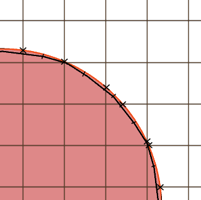
However, global optimization like that can be quite hairy to implement in real-time. A simpler approach is to compute the surface intersection point on each edge in a cell, summing them up and computing the average. The figure below shows intersection points as x's and their average - the center of mass, if you will - as dashes.
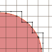
The vertex is then perturbed to the center of mass, as shown below. This turns out to work rather well. It gives a smoother mesh, while preserving sharp features by keeping vertices inside their cells.
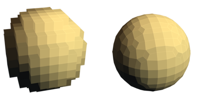
You can imagine how the technique extends itself to the third dimension. Each cell becomes a cube, and instead of linking neighbouring cells together by lines, they are connected by faces. The figure shows the process for a 3D sphere. On the left we show the mesh generated by linking together surface cells without the smoothing step. On the right, the vertices are perturbed towards the center of mass.
This naive implementation - as it is called [7] - lends itself very well to parallelization, as described in the next section.
Our GPU implementation works in three passes:
The first two passes are implemented in compute shaders, while the third pass uses a geometry shader to produce faces on-the-fly. It was easy to create links between surface cells for the 2D case above, but it might require a stretch of your imagination to do the same in 3D. So let's elaborate a bit on that.
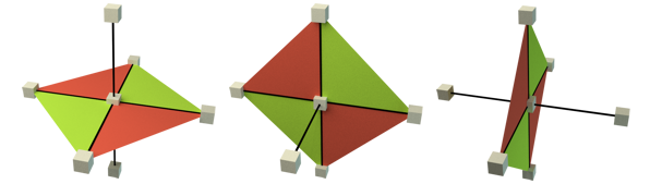
Generally, each cube on the surface can connect to its six neighbors with 12 possible triangles. A triangle is only created if both relevant neighbors are also on the surface. But considering all triangles for each cube would give redundant and overlapping triangles. To simplify, we construct faces backwards from a cube, connecting with neighbors behind, below or to the left of it. This means that we consider three edges for each cube. If an edge exhibits a sign change, the vertices associated with the four cubes that contain the edge are joined to form a quad.
To speed up the third pass, we only process cells that we know to be on the surface. This is done by the use of indirect draw calls and atomic counters. In the second pass, if the surface intersects the cell, we write the cell's index to an index buffer and increment the count atomically.
Here, N is the sidelength of the grid. When performing the draw call for the geometry shader, we bind a buffer containing the grid of points, the index buffer contaning which points to process, and an indirect draw call buffer contaning the draw call parameters.
The resulting mesh can look slightly bland. An easy way to add texture is to use an altitude-based color lookup. In the demo, we map certain heights to certain colors using a 2D texture lookup. The height determines the u coordinate, and allow for the use of the v coordinate to add some variation.

Lighting is done by approximating the gradient of the potential function in the geometry shader and normalizing, like so
This gives a very faceted look, as the normal is only computed per face. A smoother normal could be computed by approximating the gradient at each generated vertex, and blending between them in the fragment shader. Alternatively - but costly - you could sample the gradient in the fragment shader.
In this demo we have taken a look at how we can use potential functions to model complex geometry, and the rendering of such functions using mesh extraction with geometry shaders. There has been much research in the area of mesh extraction, and we have only taken a brief look at one technique.
More advanced meshing techniques, such as dual contouring [3], improve upon the shortcomings of surface nets, and allow for the use of adaptive octrees on much larger grids.
Triplanar projection mapping [2] can be used to map a texture onto all three axes of your geometry, with minimal distortion. It can add more fidelity and variation beyond simple altitude-based color lookups.
[1] Sarah F. Frisken Gibson. "Constrained Elastic Surface Nets", available online.
[2] Ryan Geiss. "Generating Complex Procedural Terrains Using the GPU", available online.
[3] T. Ju, F. Losasso, S. Schaefer, and J. Warren. "Dual Contouring of Hermite Data", available online.
[4] Paul Bourke. "Polygonising a scalar field", available online.
[5] Inigo Quilez. "Modeling with distance functions", available online.
[6] open.gl. "Geometry shaders", available online.
[7] Mikola Lysenko. "Smooth Voxel Terrain", available online.
[8] Wikipedia. "Simplex noise", available online.
[9] Wikipedia. "Perlin noise", available online.
[10] Wikipedia. "Worley noise", available online.

