 |
OpenGL ES SDK for Android
ARM Developer Center
|
|
OpenGL ES SDK for Android
ARM Developer Center
|
Using a GPU to create organic-looking 3-dimensional objects in OpenGL ES 3.0.
This tutorial demonstrates how a GPU can be used to render organic-looking 3D objects using OpenGL ES 3.0's transform feedback feature. All calculations are implemented on the GPU's shader processors. Surface triangulation is performed using the Marching Cubes algorithm. The Phong model is used for lighting metaball objects. 3D textures are used to provide access to three dimentional arrays in shaders.
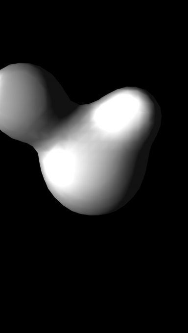
The application displays several metaballs moving in space. When the metaballs come too close to each other they smoothly change their spherical shape before becoming an organic whole. The easiest way to achieve this effect is to follow real life and use the movement of charged spheres. According to physical laws the space surrounding charged spheres will have an electrical field. Because the field at each point in space has only one value, it is often called a scalar field. A scalar field value can be trivially calculated for each point in space (a gravity field is another example of a scalar field, and is calculated using similar formulae, but applied to the weight of the spheres).
To visualize a scalar field we represent it as a surface. This is usually achieved by choosing some value level and displaying a surface containing all points in space with that chosen level. Such surfaces are usually called isosurfaces. The level value is usually chosen empirically based on visual quality.
We need to account for the capabilities of the graphics system we use to draw 3D objects. OpenGL ES can easily render 3D objects, but the only primitives useful to display surfaces that OpenGL ES accepts are triangles. Therefore, we split our model surface and represent it to OpenGL ES as a set of triangles. We have to approximate here, because a mathematically defined isosurface is smooth, whereas a surface constructed of triangles is not. We approximate the surface using the Marching Cubes algorithm.
For the Marching Cubes algorithm to work we sample the space and define the isosurface value. Marching Cubes operates on eight samples at once (one per cell corner), which form the basic cubic cell. Note that this sample uses features found in OpenGL ES3.0. In order for these features to work on your device, you must be using at least Android 4.3 or API version 18.
As with most applications dealing with 3D graphics, this example consists of several components. The Metaballs project is constructed from five components: one control program that is run on the CPU and four supplementary shader programs run on the GPU. Usually, programs run on a GPU consist of two parts: a vertex shader and fragment shader. In this example we use eight shaders (two for each stage), but only five shaders contain actual program code; the remaining three shaders are dummy shaders required for the program object to link.
We split the application into the following stages:
We use transform feedback mode in the first three stages. The transform feedback mode allows us to capture output generated by the vertex shader and to record the output into buffer objects. Its usage is explained in detail in Calculation of sphere positions. All four stages are executed for each frame in the rendering loop. Additionally, each stage requires some initialization operations that are executed in the setupGraphics() function of the control program.
Because the whole scene depends on the sphere positions at the currently rendered time, we need to update the positions as a first step. We can keep information describing spheres and their movement equations in the vertex shader, because for further calculations we need only the current sphere positions. This enables us to improve overall performance by minimizing amount of data transferred between CPU and GPU memory. The only input information required for the vertex shader of this stage (spheres_updater_vert_shader) from the control program is the time value, which we declare in the vertex shader as a uniform:
To pass values from the control program to the shaders, we retrieve a location for the uniforms once the shader program is compiled and linked. For this stage we need to retrieve only the location of the time uniform in the setupGraphics() function:
During the rendering loop we pass the current time value to the vertex shader with a command:
Now let's take a look at the output values generated in this stage by the vertex shader:
As you can see in its source code, the shader outputs only four floating point values (packed as vec4s): three sphere coordinates and a sphere weight. To calculate parameters for n_spheres spheres, we instruct OpenGL ES to run the vertex shader n_spheres times. The control program does this by issuing the command during the rendering loop:
As the calculations of sphere positions are independent of each other, OpenGL ES might (and most often does) run calculations for several spheres at the same time on multiple vertex processors.
Capturing values produced by the vertex shader require us to specify in the control program which varyings (that is, shader output variables) we are interested in before linking the program:
Here we specify that we are interested in one value, which is defined in the sphere_position_varying_name constant.
Each calculated sphere position is written into an appropriate place in a buffer attached by the control program. In the setupGraphics() function we need to allocate a buffer object and allocate a storage to store values generated by the shader:
Next, we allocate a transform feedback object (TFO), and configure it by binding an appropriate buffer object (in this case spheres_updater_sphere_positions_buffer_object_id) to the GL_TRANSFORM_FEEDBACK_BUFFER target:
In these lines we tell OpenGL ES to store the output values in the buffer when transform feedback mode is activated. This TFO is activated by binding it to the GL_TRANSFORM_FEEDBACK target. That's exactly what we do as the first step during the rendering process:
After that, we need to prepare the transform feedback mode to be useful for our purposes: we don't need primitives to be rendered at this stage and we want to capture data. The first command shortens the OpenGL pipeline by discarding any primitives generated by the vertex shader:
The second command activates the transform feedback mode itself, instructing OpenGL ES to capture and store the specified primitives into the buffer object:
When we're done, we issue paired commands to deactivate transform feedback mode:
And another to restore the OpenGL ES pipeline:
To sum up, here is the complete listing for this stage:
There are very few differences in the control program between this stage and the first stage:
Although we use different program, buffer and transform feedback objects, the general flow of operations in the control program is the same as the first stage. This is because at this stage we again use the transform feedback mechanism and only need to specify input and output variables to vertex shader, which will do the actual work. The only differing command is the first one, which binds the buffer object to GL_UNIFORM_BUFFER target. By issuing this command we make the sphere positions that were generated and collected in the buffer object during the first stage available to the vertex shader at this stage. Unfortunately, only a relatively small amount of data can be passed to shaders using this mechanism due to limitations in OpenGL ES. It is also worth noticing that we instruct OpenGL ES to run the shader program samples_in_3d_space times, which will be explained below.
The main difference is in the stage's vertex shader, which we'll examine after looking at the ideas of the stage.
As you know, the gravity field value generated by an object with mass M in a point in space at distance D from the object directly correlates with that mass and square of that distance, i.e. FV=M/(D2). In order to have a physical meaning for this formula we also need to introduce a constant coefficient, but for the purposes of this example it can be omitted. The gravity field value generated by multiple objects is calculated as sum of all field values, i.e. FVtotal=ΣFVi. In this example we'll use term weight instead of mass, which while not as correct as mass is usually easier to understand.
It is hard to deal with surfaces as defined mathematically, so as in many other sciences we simplify the task by sampling the space. We use tesselation_level=32 samples for each axis, which provides us with 32*32*32 or 32768 points in space for which a scalar field value should be calculated. You may try to increase this value to increase the quality of the image generated.
If you take a look at the forumlae above, you may notice that the scalar field value depends only on the positions and masses (weights) of all spheres. This enables us to calculate the field value for several points in space at the same time in different shader programs.
As input data, the vertex shader expects the number of samples on each axis and the sphere positions stored in the buffer:
As you can see, the number of spheres stored in buffer is hardcoded here by using a preprocessor define. That's the limitation of shaders: they need to know the exact number of items in the incoming uniform buffer. If you need to make shader more flexible, you may reserve more space in the buffer and ignore items based on some flag or by validating some value (for example zero weight value). Another approach is to use a texture as input array of data, which we will use in Scalar field generation.
Each vertex shader run in this stage starts execution by decoding the point in space for which the shader is running:
This is a quite widely used technique where the built in OpenGL ES Shading Language variable gl_VertexID is used as an implicit parameter. Each executed vertex shader has its own unique value passed via gl_VertexID with the range zero to the value of the count parameter passed into the glDrawArrays call. Based on the gl_VertexID value, the shader can control its execution appropriately. In this function the shader splits value of gl_VertexID into x, y, z coordinates of point in space for which the shader should calculate the scalar field value.
To make a scalar field value independent from the tesselation_level, the shader normalizes the point in space's coordinates to the range [0..1]:
It then calculates the scalar field value:
And finally the shader outputs the calculated scalar field value using the only output variable declared in the shader:
At the end of this stage we have scalar field values calculated and stored in the buffer object for each point in space. Unfortunately, large buffer objects cannot be used as input data. That's why at the end of this stage we need to perform one more operation: we apply another widespread OpenGL ES technique and transfer the data from the buffer object into a texture. This is performed in the control program:
The first command above activates texture unit one, the second command specifies the source data buffer, and the third command performs the actual transfer of data from the buffer object into the texture object currently bound to the GL_TEXTURE_3D target at a specific binding point. We use the 3D textures as a convenient way to access the data as a 3D array in the next shader stage.
The texture bound to the GL_TEXTURE_3D target point of texture unit one is created and initialized to contain an appropriate number of scalar field values in the setupGraphics() function:
The last two stages actually implement the Marching Cubes algorithm. The algorithm is one of the ways to create a polygonal surface representation of a 3D scalar field isosurface [1], [2]. The algorithm breaks the scalar field into cubic cells. Each cell corner has one scalar field value. By performing a simple compare operation between the isosurface level and the scalar field value in the cell corner, it can be determined whether the corner is below the isosurface or not. If one corner of a cell is below the isosurface and another corner on same cell edge is above the isosurface then obviously the isosurface crosses the edge. Also, due to field continuity and smoothness, there will be other crossed edges in same cell. Using edge cross points, a polygon can be generated that will best approximate the isosurface. Now let's take a look at the algorithm from the other side. The state of each cell corner can be represented as a boolean value: either the corner is above the isosurface (appropriate bit set to 1) or not (appropriate bit set to 0). It is obvious that having eight corners in a cell we have 28, i.e. 256 cases where corners are either above or below the isosurface. If a surfaces passes straight through a corner we assume the corner is below the isosurface, to keep the state binary. In other words, the isosurface can pass through the cell in one of 256 ways. Thus with 256 cell types we can describe a set of triangles to be generated in order for the cell to approximate an isosurface.
At this stage we divide the space by the cells and identify cell types. The space was already divided by samples at a previous stage (Scalar field generation) and the shader takes eight samples in cell corners to form a cell. Using the isosurface level value, the shader identifies a cell type for each cell according to the algorithm described above.
Stage three of the control program is even closer to the stage two control program, so we won't describe the whole thing. We will, however, pay some attention to texture creation in the setupGraphics() function:
Notice that here we use texture unit two and create a 3D texture of one-component integers (GL_R32I), which will hold types for each of the 31*31*31 cells. The number of cells on each axis (cells_per_axis) is one less than the number of samples on each axis (samples_per_axis). It is easier to explain why using an example: let's imagine that we cut a butter brick into two halves (cells). Parallel to the cut plane we have three sides for two cells (one is shared by both halves). Thus the number of cells is one less than the number of sides. The control program instructs the GPU to execute the vertex shader for each cell:
In this stage's vertex shader we first decode the position in space of the origin point of the cell processed by this instance of the shader in a way similar to what we did in the previous stage. The only difference is that here as a divisor, we use the number of cells on each axis and not the number of samples:
The shader then gathers the scalar field values for the corners of current cell into an array by extracting scalar values from the texture, which was created during the previous stage (Scalar field generation):
Having the values of the scalar field in the cell corners, and the isosurface level value, we can determine the cell type:
The cell type is returned by this stage and stored in an appropriate buffer for further processing during the next stage.
The Marching Cubes algorithm approximates a surface passing through the cell with up to five triangles. For cell types 0 and 255 it generates no triangles, due to the fact that all the cell corners are either below or above the isosurface. Using a lookup table indexed by cell types (tri_table) is an efficient way to get a list of triangles generated for the cell.
Finally, we have all the information needed to generate a set of triangles and to render them. For this stage the control program does not activate transform feedback mode, because there is no need to store any generated triangle vertices. It is more useful to pass the generated triangle vertices to the fragment shader for culling or rendering:
If you take a look at the constant values, you might notice that here we instruct OpenGL ES to run the shader fifteen times for each cell. This multiplier comes from the Marching Cubes algorithm: an isosurface passing through a cell and intersecting each edge no more than once can be approximated with up to five triangles, and we use three vertices to define one triangle. Notice also that the algorithm does not use the cell corners to build triangles, but instead uses the "middle" points of the cell. In this case, the "middle" point is a point on the cell edge where that edge is actually intersected by an isosurface. This provides better image quality.
Each cell can produce maximum of five triangles according to its cell type, but most of the cell types produce significantly fewer triangles. For an example, look at tri_table, which is used to build triangles out of cell types. We present first four cell types out of 256 here:
Each row in the table represents one cell type. Each cell type contains up to five triangles. Each triangle is defined by three sequential vertices. Each number in the table is a number of a cell edge, of which the "middle" point is taken as a triangle vertex. If the cell type provides fewer than five triangles, then the extra edge numbers are filled with the value -1. For example, cell type 0 (first data line) does not define any triangles: all of its "middle" points are set to -1. Cell type 1 (second data line) defines one triangle consisting of the "middle" points of edges 0, 8 and 3 of a cell. Cell type 2 defines a single triangle again, while cell type 3 defines two triangles. An observant reader might notice that the number of cell edges in the table is less than 12. This is because the cell cube has only 12 edges, which are numbered in the table from 0 to 11 inclusive.
Each vertex shader instance processes only one vertex of a triangle. At first, based on gl_VertexID it decodes the triangle vertex number and the position of the cell it processes in a way similar to Scalar field generation :
Here, the decoding is one step longer: besides the cell coordinates it also decodes the combined triangle and vertex number. We store this information in the main() function's local variables for further processing:
Having obtained coordinates, the shader can retrieve cell type and cell edge number:
From here we proceed only if the shader should generate a vertex (i.e. the edge number is not equal to -1). The discarding of dummy triangle vertices will be considered later.
From the cell coordinates we can calculate the coordinates of the origin point of the cell:
Having coordinates of the cell origin point and the edge number (of which "middle" point we are currently calculating), we can find the cell corner vertices at which this particular edge begins and ends:
Now, having the values of the scalar field in the beginning and end vertices of the edge and the isosurface level value we can calculate the exact position at which the isosurface crosses the edge:
And for lighting we calculate a normal vector to the isosurface:
The normal vector to the surface in the edge "middle" point is calculated as a mixture of normal vectors in the beginning and end edge vertices. The normal vector in the beginning and end edge vertices is calculated using partial derivatives of the scalar field, which are calculated using the scalar field values adjacent to the vertex scalar field values. For more information on calculating a normal vector to a surface please take a look at [3]. It is assumed that you are already familiar with this lighting technique, so we will not focus on describing the effect in detail.
If it turns out that the shader processes a vertex of a triangle that should not be generated (the edge number is -1), then it drops processing the vertex by specifying coordinates that match all other vertices of the dummy triangle:
It would be more optimal to use a geometry shader for this stage, which (unlike a vertex shader) could generate as many vertices as required, or none at all. However, geometry shaders are an OpenGL feature and not present in core OpenGL ES, so we need to do the job in a vertex shader, discarding inappropriate triangles by specifying all their vertex coordinates to the same value.
The fragment shader implements a simple Phong lighting model [4]. For more information, look at the code comments in the fragment shader of the Marching Cubes triangle generation and rendering stage.
[1] http://paulbourke.net/geometry/polygonise/
[2] http://en.wikipedia.org/wiki/Marching_cubes
[3] http://mathworld.wolfram.com/NormalVector.html
[4] http://en.wikipedia.org/wiki/Phong_shading

