This sample uses OpenGL ES 3.0 and Pixel Local Storage to perform advanced shading techniques. The sample computes a per-pixel object thickness, and uses it to render a subsurface scattering effect for translucent geometry, without the use of external depth-maps or additional rendertargets.

Introduction

This sample uses OpenGL ES 3.0 and the Pixel Local Storage extension to perform advanced shading techniques. A two-pass routine is used to calculate a per-pixel object thickness, and stores it together with material properties in fast on-chip memory known as local storage. The thickness data is used in a deferred shading pass to approximate effects of translucency and subsurface scattering. For efficiency, the stencil buffer is used to mask out relevant objects when computing thickness and performing shading. Finally, the translucent geometry is rendered together with opaque geometry.

The source code for this sample can be found in the folder of the SDK. Feel free to read along with the documentation.

Translucency and subsurface scattering

Translucency is the effect of light passing slightly through a material. It is inbetween two extremes - opaque (no light passes through) and transparent (all light passes through). Many materials are somewhat translucent. Light has a tendency to bounce around rather sporadically inside such materials, and brighten parts that were not directly lit in the first place. This effect is called subsurface scattering, and is the holy grail for skin-rendering enthusiasts, but is also relevant for materials such marble, leaves, wax and milk.

As expected, much research effort has been put into how to compute realistic subsurface scattering. In this sample we do the opposite, and aim for the roughest of rough approximations, intended for use when performance is of greater concern than realism. We'll show how you can easily combine the technique with traditional deferred rendering, using the pixel local storage extension. Since we don't rely on additional rendertargets, we also achieve better performance on bandwidth-limited devices, such as mobiles.

Approximated translucency shading

Recent work for real-time approximations tend to use texture-space blurring or rely on additional depth-maps. While these techniques tend to look quite good, they may require significant amounts of memory and moving around of said memory. This is bad for mobile devices, so we'll try not to do that. Instead, this sample will forego the usage of external depth- and texture maps, and rely purely on fast, on-chip local storage. The downside to this is that the effect can become slightly limited, and will therefore be a very, very rough approximation of how scattering works in real-life.

The scattering model we apply is based on Colin Barré-Brisebois' GDC presentation, "Approximating Translucency for a Fast, Cheap and Convincing Subsurface Scattering Look" [6]. Simply put, light is attenuated as it travels through a material. And the attenuation is influenced by many things, such as the varying thickness of the object, the view direction and the properties of the light.

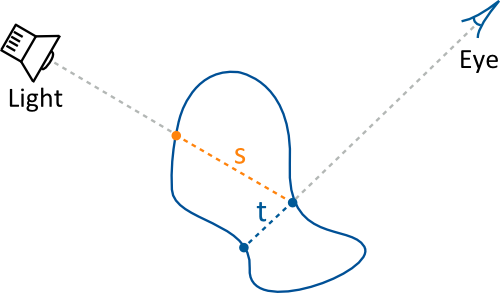
Computing per-pixel object thickness

In order to perform the shading effect described above, we need to determine how far the light travels inside an object before it reaches the point to be shaded. We approximate this distance by computing the object thickness as seen from the camera, instead of the actual distance travelled by the light. The above mentioned technique uses precomputed thickness maps, but we will compute the object thickness during runtime. Computing the thickness in runtime has the additional benefit of supporting deformation, which may be relevant for dynamic materials such as jelly or milk. To make matters clear, the figure below shows the per-pixel object thickness we compute, t, versus the actual distance the light travels, s.

The thickness is computed by taking the difference between the maximum and the minimum view-space depth of an object. To simplify matters, we'll only consider the closest object to the camera and assume that the effect of background objects is negligible. This assumption might not hold, but it does prevent overestimating the thickness, which would be a much more apparent artifact. To compute the thickness we use two shader passes.

The first pass is used to determine what the closest object is, and its minimum view-space depth. We render each translucent object with depth testing, and set a unique object identifier in the stencil buffer. Since depth testing is enabled, we can be sure that the final fragment will belong to the closest object. The object ID is simply an integer, greater than 0, that we use in the second pass to determine the max depth for the closest object. For convenience, we reserve the ID of 0 to distinguish translucent geometry from opaque geometry. The view-space depth is stored in pixel local storage, together with material properties in the following layout.

__pixel_localEXT FragDataLocal {
    layout(rgb10_a2) vec4 lighting; // RGBA
    layout(rg16f) vec2 minMaxDepth; // View-space depths
    layout(rgb10_a2) vec4 albedo;   // RGB and sign(normal.z)
    layout(rg16f) vec2 normalXY;    // View-space normal components
} storage;

The fragment shader for this pass writes the material properties and sets both minimum and maximum depth to be the incoming depth. We also clear the lighting variable, which will be used to accumulate lighting in the shading pass later.

uniform vec3 albedo;
in vec4 vClipPos;
in vec4 vPosition;
in vec3 vNormal;
void main()
{
    vec3 n = normalize(vNormal);
    storage.lighting = vec4(0.0);
    storage.minMaxDepth = vec2(-vPosition.z, -vPosition.z);
    storage.albedo.rgb = albedo;
    storage.albedo.a = sign(n.z);
    storage.normalXY = n.xy;
}

The second pass finds the maximum depth of the previously determined closest object. To do this we render the same objects again - without depth testing - but with a stencil test set to equal each object's ID. Since the ID of the closest object is stored in the stencil buffer, only that same object will have fragments that pass through. We can then do a max of the stored max-depth and the incoming depth.

void main()
{
    float depth = -vPosition.z;
    storage.minMaxDepth.y = max(depth, storage.minMaxDepth.y);
}

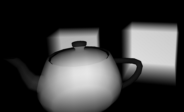
The figure below shows the resulting object thickness when applied to a scene of two boxes and a teapot.

Shading pass

Once the material properties and the view-space thickness have been computed and stored in the local storage, we can perform a shading pass over all translucent geometry. We can use the previously written stencil buffer values for extra efficiency here. By setting the stencil test function to only pass whenever the stored value is greater than zero, we can avoid running the costly lighting computation for fragments that don't contain any translucent geometry. Now let's examine the shader used for the translucency effect.

vec3 lighting(vec3 P, vec3 Lp, vec3 N, vec3 V, float thickness, float Li, vec3 Ldiff, vec3 Cdiff)
{
    // Compute distance to light from point being shaded
    float r = length(P - Lp);
    // Apply Blinn-Phong shading model
    // float Iblinn = ...
    // Apply subsurface scattering
    thickness = min(thickness, r);
    float Isss = sss(P, L, V, N, r, thickness);
    
    // Compute attenuation
    // float attenuation = ...
    return attenuation * (Iblinn + Isss) * Ldiff * Cdiff;
}

First, we compute a standard Blinn-Phong lighting contribution. It will be the prevalent shading when the point being shaded is directly visible from both the light source and the viewer. The next thing we do is to take the minimum of the object thickness and the distance to the light from the shading point. This is done to prevent overestimation of the distance that the light travels through the material. It also blends rather nicely into the case where lights are inside objects. Next we compute the translucency term.

float sss(vec3 P, vec3 L, vec3 V, vec3 N, float r, float thickness)
{
    vec3 Lt = -(L + N * distortion);
    float VdotL = pow(clamp(dot(V, Lt), 0.0, 1.0), sharpness) * scale
    return (VdotL + ambient) * clamp(1.0 - thickness * 0.5, 0.0, 1.0);
}

The basic idea is that thickness attenuates light transmittance. When the thickness is large, the transmitted light intensity will be close to zero. When the object is very thin, the intensity will be somewhat larger. We refer to [6] for more details regarding this lighting model.

Suffice to say, the model first computes the inverted light vector and distorts it by the surface normal. The resulting vector is then dotted with the direction to the viewer, so that light is most prevalent when going through the material and towards the viewer. Similarly to how you would compute a specular, the dot product is raised to a power we denote as sharpness. This controls how focused the light will be.

(The call to pow might shock and horrify most readers, but rest assured, it is optimized in the actual code. See [7] for details.)

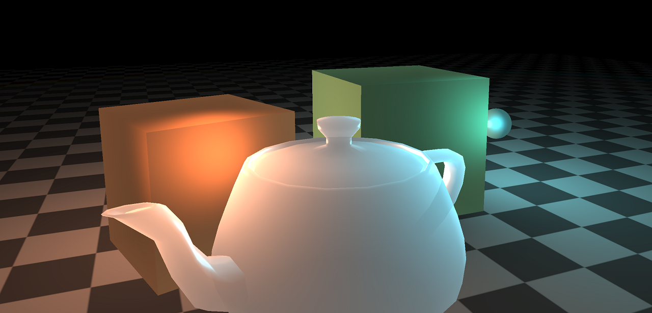
There are several interesting parameters that can be adjusted to achieve different visual results. For example, the image below shows the same scene, but adjusted such that the objects transmit less light. A more thorough comparison can be found in [6].

References

[1] Khronos. "EXT shader pixel local storage", available online.

[2] Marius Bjørge and Sam Martin. "Bandwidth-efficient graphics", available online.

[3] Jan-Harald Fredriksen. "Pixel Local Storage on ARM® Mali™ GPUs", available online.

[4] Jorge Jimenez and David Whelan and Veronica Sundstedt and Diego Gutierrez. "Real-Time Realistic Skin Translucency", available online

[5] Henrik Wann Jensen and Stephen R. Marschner and Marc Levoy and Pat Hanrahan. "A Practical Model for Sursurface Light Transport", available online

[6] Colin Barré-Brisebois and Marc Bouchard. “Approximating Translucency for a Fast, Cheap and Convincing Subsurface Scattering Look”, GDC 2011, available online.

[7] Colin Barré-Brisebois. "Simplified Spherical Gaussian Exponentiation", available online.