Occlusion Culling with Hierarchical-Z

This sample will show you how to efficiently implement occlusion culling using compute shaders in OpenGL ES 3.1. The sample tests visibility for a large number of instances in parallel and only draws the instances which are assumed to be visible. Using this technique can in certain scenes give a tremendous performance increase.

Introduction

Note

This sample uses OpenGL ES 3.1.

This sample assumes basic knowledge of OpenGL ES compute shaders and OpenGL ES 3.0. Some important features for this sample:

• Shader storage buffer objects (SSBOs)
• Atomic operations
• Indirect drawing
• textureGather() (GLSL)

Problem

Sometimes an application will want to manage a large number of instances of an object. These instances might be fully dynamic and controlled by the GPU using OpenGL ES 3.1 compute shaders. Eventually, we want to draw these instances, but depending on our scene, only a small number of instances might actually be visible at one time due to various occluders in our scene.

Depending on the number of objects in our scene, drawing every instance regardless of visibility could be very taxing on performance, and determining visibility on CPU might not be practical.

Considering OpenGL ES 3.0 Occlusion Query

OpenGL ES 3.0 has the occlusion query functionality which lets you determine visibility of a draw call. It does however, have some shortcomings in this case.

• Instancing not supported. Would need one query object per instance.
• Readback to CPU is required.

The usage scenarios for occlusion query tend to be simpler, with fewer meshes.

Test scene

In this test scene, we have chosen a simple scene to demonstrate the problem, and how the occlusion culling technique provided here can help solve it.

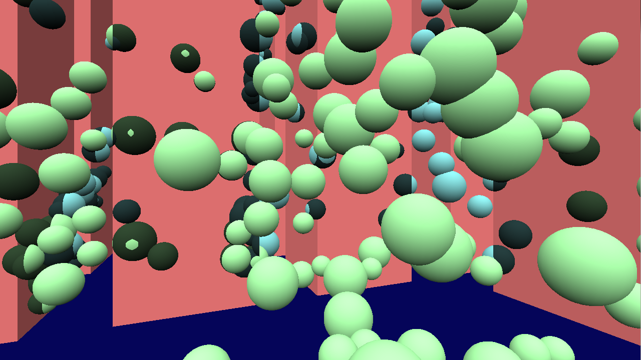
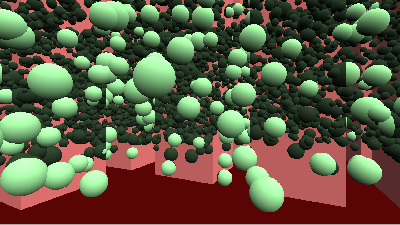
For simplicity the sample meshes are spheres and occluders are modeled as tall prisms. We will draw the scene twice. One time to draw the spheres, and once to draw the spheres with a GL_GREATER depth test to visualize the spheres which are redundantly drawn causing lots of extra vertex shading work. Spheres which are redundantly drawn are drawn with a darker color.

Without any form of culling, we see the scene is completely dominated by invisible objects.

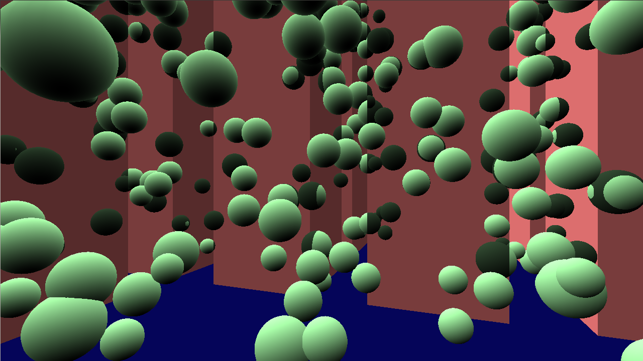
However, using the techniques described below, we can reduce this to a far more manageable amount.

Hierarchical-Z

The main idea of Hierarchical-Z is to represent the depth of a scene with multiple resolutions. Using multiple depth map resolutions, we can quickly and efficiently determine visibility of an instance.

Rendering the depth of the current scene is a fixed cost, but cost of testing visibility for a single instance is made very low.

Rendering Hierarchical-Z depth map

First, we need to separate our scene into occluders and occludees. Occluders will be big objects which naturally occlude other objects.

Occluders can if desired be represented with low-poly occlusion geometry. The requirement for occlusion geometry however, is that it must not contain any volume not already contained by the original mesh. This is to avoid falsely discarding visible instances.

Note

Occluder geometry is opposite of bounding boxes. Bounding boxes must contain all volume the original mesh does, but occluder geometry cannot contain any volume outside the mesh.

Occludees can also be used as occluders if occludees tend to occlude themselves. The same rules for occlusion geometry applies.

We render these to a low-resolution depth texture (256x256 for example). To represent the scene depth at various resolutions, we can mipmap our depth texture down to a 1x1 texture. Since depth textures are not filterable, we manually mipmap the depth texture. To conservatively represent the scene depth at a larger resolution, we have to use a max() filter on our depth. In OpenGL ES 3.1, we can use the new textureGather() function to obtain all four depth values in a quad in one texture lookup.

void main()
{
    vec4 depths = textureGather(uDepth, vTex, 0); // Get depth values from all surrounding texels.
    gl_FragDepth = max(max(depths.x, depths.y), max(depths.z, depths.w)); // Write conservative depth.
    gl_FragColor = vec4(1.0); // Ignored
}

For reference, there are some sample depth maps below which are mipmapped using this approach.

Note

By rendering scene depth to a lower resolution than the actual scene we do risk falsely culling instances. However, this edge case can only possibly occur when a few pixels from an object are visible. Bounding volumes tend to be a bit larger than the actual object itself, which makes this case even more unlikely. In a real application, such a case would normally not be significant enough to warrant rendering the scene depth in full resolution, but if it does become an issue, the resolution can always be increased as needed. Alternatively, using conservative rasterization can be considered, but the implementation complexity would drastically increase.

Filtering data sets with compute shaders

Occlusion culling is essentially a filtering operation. From a set of data, we include elements in the filtered set based on a condition. Before going into the particular occlusion culling technique, it's useful to look at filtering data with compute shaders in general.

Compute shaders (and GPUs) run in parallel, which means the obvious serial approach does not work, e.g.:

for (auto &data : dataset)
{
    if (predicate(data))
    {
        filtered_dataset.push_back(data);
    }
}

Instead, we could use atomic counters to allow the loop bodies to run fully in parallel, here expressed with C++11-style atomics:

std::atomic_uint counter{0};
for (auto &data : dataset)
{
    // Assume loop body runs in parallel.
    if (predicate(data))
    {
        // Due to the nature of atomic adds,
        // every value obtained must be unique, and it's hence
        // safe to do this loop fully in parallel.

        // NOTE: On a CPU implementation, we would probably implement this very differently,
        // this is just to illustrate the point.
        unsigned int unique = counter.fetch_add(1, std::memory_order_relaxed);

        // filtered_dataset must be preallocated to hold at least
        // dataset.size() elements.
        filtered_dataset[unique] = data;
    }
}

// Synchronize all threads.

Data will be added to the filtered dataset unordered due to parallelism, but this is not a problem for occlusion culling.

We can translate the C++11-style example to compute shaders, where it would look something like:

#version 310 es
layout(local_size_x = 1) in;
layout(std430) buffer;

struct InstanceData { ... };

bool predicate(InstanceData data)
{
   ...
}

layout(binding = 0) buffer InputData
{
    readonly InstanceData data[];
} dataset;

layout(binding = 1) buffer OutputData
{
    writeonly InstanceData data[];
} filtered_dataset;

// Can also do atomic operations on an SSBO.
layout(binding = 0, offset = 0) uniform atomic_uint instanceCount;

void main()
{
    uint ident = gl_GlobalInvocationID.x;
    InstanceData data = dataset.data[ident];

    if (predicate(data))
    {
        uint unique = atomicCounterIncrement(instanceCount);
        filtered_dataset.data[unique] = data;
    }
}

If we now consider the occlusion culling case again, we can consider something like:

struct InstanceData { ... };

bool is_instance_visible(InstanceData data)
{
    // Hierarchical-Z test here.
}

layout(binding = 0) buffer InputData
{
    readonly InstanceData data[];
} instance_data;

layout(binding = 1) buffer OutputData
{
    writeonly InstanceData data[];
} filtered_instance_data;

// Can also do atomic operations on an SSBO.
// instanceCount in indirect draw buffer is found at offset = 4.
layout(binding = 0, offset = 4) uniform atomic_uint instanceCount;

void main()
{
    uint ident = gl_GlobalInvocationID.x;
    InstanceData data = instance_data.data[ident];

    if (is_instance_visible(data))
    {
        uint unique = atomicCounterIncrement(instanceCount);
        filtered_instance_data.data[unique] = data;
    }
}

Hierarchical-Z Visibility Test

The Hierarchical-Z visibility test is implemented here as a single compute shader. It will read a buffer of bounding volumes represented as bounding spheres or bounding boxes and output a tightly packed instance buffer as well as a counter for the number of elements in the buffer.

Frustum Culling Pre-pass

Before attempting any kind of Hi-Z culling, we first attempt to frustum cull the instance. Frustum culling is implemented very efficiently (especially for bounding spheres), and by frustum culling, we also avoid some edge cases with the Hi-Z algorithm later.

See the Terrain OpenGL ES 3.0 sample for more detail on how frustum culling can be implemented.

Computing Screen Space Bounding Box

Since we need to base our visibility decision on a 2D depth map, we must project our instance down to a screen space bounding box first. It is important that the bounding box is as small as possible to avoid overconservative culling.

For axis-aligned bounding boxes, projecting a bounding box is fairly straight forward. We can take the 8 corners and project them to screen, then take min/max of screen space X/Y and use the minimum Z as our reference depth value against depth map. The only edge case we have to handle here is when the bounding box intersects with the near plane. We then risk dividing by w <= 0.0, which will give us unexpected results. To avoid this case, we can treat all instances which intersect the near plane as visible. An object so close to the screen that it clips will likely be visible anyways.

For bounding spheres, the screen space bounding box computation is more complicated as there are no corners that can be transformed and projected. We have to take into account perspective warping that happens when the spheres move away from the center of the screen as well. In this sample, we focus on bounding spheres as occlusion testing is significantly cheaper than testing bounding boxes. We implemented the simplest case of the algorithm in [1]. To find minimum Z value, we perform a view transform of the bounding sphere center, add radius to Z, and perform a perspective transform of the Z coordinate.

Visibility Testing

When we know the screen space bounding box for an instance and minimum Z, we can test against our depth texture.

We first find a mip-level where four depth texture texels covers the entire screen space bounding box. We can then do a single PCF depth compare lookup to test these four texels. If PCF result is > 0.0, at least one texel compared to 1.0 and we must assume the instance is visible.

See implementation for more details.

Indirect Drawing

After culling our scene we have a count of number of visible objects due to atomic increments, and a tightly packed array of visible instance data.

The instance count is currently not known to the CPU yet as the atomic count is backed by a GL buffer. We can perform an indirect draw which lets us perform a draw call with unknown parameters. E.g.:

glBindBufferBase(GL_ATOMIC_COUNTER_BUFFER, 0, indirect_buffer);
glBindBufferBase(GL_SHADER_STORAGE_BUFFER, 0, instance_buffer);
glBindBufferBase(GL_SHADER_STORAGE_BUFFER, 1, filtered_instance_buffer);
do_occlusion_culling(...);
glMemoryBarrier(...);

glBindVertexArray(instance_vertex_array);
glBindBuffer(GL_DRAW_INDIRECT_BUFFER, indirect_buffer);
glDrawElementsIndirect(...); // We don't know instanceCount on the CPU, but GPU knows.

OpenGL expects a fixed layout of the buffer object to read data like element count, instance count, base vertex, etc. See OpenGL ES 3.1 reference or the code for details.

Considerations for occlusion culling meshes belonging to different draw calls

In real-world scenes, not every mesh can be instanced, which makes this technique more difficult to implement efficiently, because we would need several indirect draw calls.

One possibility is instead of filtering per-instance data, one can compute a visibility buffer where each mesh gets a 0/1 value. A readback to CPU could be done where the application will draw meshes depending on GPU computed results. This is inoptimal due to GPU-to-CPU readback which can break pipelining. A workaround for pipelining issue would be to readback older results, but culling results could be incorrect if camera or objects have moved significantly. A more advanced workaround for the pipelining issue would attempt some kind or reprojection, but this is outside the scope of this sample.

Overall, this technique is most efficient for cases where you cull instances belonging to the same instanced draw call.

Sorting instances in level-of-details

A common technique for reducing shading load is to recognize that objects far away from the camera require less detail. It is possible for artists to create meshes with different detail levels which can be drawn according to quality needs. We can employ this idea for occlusion culling as well.

In the compute dispatch doing culling, we already know the minimum depth value for the bounding volume. We can simply partition the depth space into a fixed number of regions. Our shader code would look something like this for four level-of-details.

// Number of atomic_uints we can use is limited.
// Could use atomics on a single SSBO if we need many LODs.
layout(binding = 0, offset = 4) uniform atomic_uint lod0Counter;
layout(binding = 1, offset = 4) uniform atomic_uint lod1Counter;
layout(binding = 2, offset = 4) uniform atomic_uint lod2Counter;
layout(binding = 3, offset = 4) uniform atomic_uint lod3Counter;

// depth is the non-linear device space depth.
void append_instance(InstanceData data, float depth)
{
    if (depth > 0.9)
    {
        uint count = atomicCounterIncrement(lod3Counter);
        instance_data_lod3.data[count] = data;
    }
    else if (depth > 0.8)
    {
        // And so on ...
    }
}

In GL, we end up with four indirect buffers and four instance buffers. We split this up into four different indirect draw calls where we instance over meshes of different quality levels. We can even use different shaders for the draw calls. A mesh that is far away might not require normal mapping for example.

Another added benefit of sorting like this is that objects close to the screen can be drawn first (LOD0), which makes sure objects are drawn approximately front-to-back, enabling early-Z optimizations.

In this sample, we implement both the single LOD, and multiple LOD approaches. LODs farther away from the camera are drawn with a blue-ish tint.

Single LOD.

Multiple LODs.

References

[1] http://jcgt.org/published/0002/02/05/paper.pdf