This sample illustrates how to efficiently perform calculations on a large amount of particles using OpenGL ES 3.1 and compute shaders.

Introduction

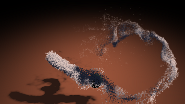
This sample uses OpenGL ES 3.1 and compute shaders to seamlessly advect tens of thousands of particles. We use a combination of potential flow theory and procedural noise, to simulate the turbulent wake of smoke moving around an interactive object. After simulation, the particles are sorted using a GPU-accelerated radix sort, and then rendered as alphablended sprites with volumetric shadows.

The source for this sample can be found in the folder of the SDK.

A brief introduction to fluid dynamics

We simulate the flow by generating a velocity field for our scene. The velocity field is a 3D vector function, which tells us how fast a particle is moving at any point in space. For fluids that are incompressible, it's important that this field is divergence-free. This is the mathematical way of saying that the particles don't clump together into a single spot or drift far apart anywhere.

Luckily for us though, it turns out that we can find such a field easily with some clever mathematics! First of all, our field will consist of two parts. The first is a repulsive component close to the object that will push the smoke away. We generate this by using a source potential from ideal-flow theory, which is a scalar function defined as

phi = -a * ln(r + e)

where r is the distance from the origin of the point evaluated. The velocity can be computed directly by taking the gradient of this function. The result is a field which is divergence-free everywhere but the origin. To eliminate the singularity at the origin, we add a small epsilon term e.

The second component is crucial for a good looking particle system - a procedural 3D noise field. This adds turbulent movement to our particles, which makes it overall much more exciting. It can be shown that if we use a noise function which is smooth (in the mathematical sense), the curl of this field becomes a divergence-free vector field. This is the curl noise method described in [2]. In the demo we use simplex noise to generate the field, and calculate the partial derivatives analytically. Stefan Gustavson explains how simplex noise works in his paper [14]. He also cooperated on a fast, vectorized, non-branching GLSL version ([15] [16]).

The final velocity field is simply the sum of the two components. Further details about the curl noise technique, and interesting extensions to it, can be found in [2].

Storing the particle data

To simulate the particles we need to keep track of their position in space. In addition, we give each particle a certain lifetime, which decreases over time. When the life runs out, the particle respawns at a semi-random location around an emitter. We store this information in shader storage buffer objects, which are special buffers that can be both read from and written to inside the compute shader.

void init_particles()
{
        vec4 *data = new vec4[NUM_PARTICLES];
        for (int i = 0; i < NUM_PARTICLES; ++i)
        {
                vec3 p = random_position();
                float lifetime = PARTICLE_LIFETIME;
                data[i] = vec4(p, lifetime);
        }
        glGenBuffers(1, &position_buffer);
        glBindBuffer(GL_SHADER_STORAGE_BUFFER, position_buffer);
        glBufferData(GL_SHADER_STORAGE_BUFFER, NUM_PARTICLES * sizeof(vec4), data, GL_DYNAMIC_DRAW);
        glBindBuffer(GL_SHADER_STORAGE_BUFFER, 0);
        delete[] data;
}

Note that since we only need three components to store the position, we can fit the lifetime parameter in the w-component of a vec4. Thus we only need a single buffer and we get a slight speedup by having fewer lookups in the shader.

Simulation

The advection of the particles is done in a single-pass compute shader. Advection is the flow of the particles. For each particle, we evaluate the velocity field at the particle's position, and do simple Euler-integration to forward the simulation. Because each particle is independent from the rest, this type of simulation is a perfect job for the GPU. The simplified code below shows how the update shader works.

#version 310 es
layout (local_size_x = 64) in;
layout (std140, binding = 0) buffer ParticleBuffer {
        vec4 Particle[];
};
layout (std140, binding = 1) buffer SpawnBuffer {
        vec4 SpawnInfo[];
};
// ...
void main()
{
        uint index = gl_GlobalInvocationID.x;
        vec4 status = Particle[index];
        vec3 position = status.xyz;
        float lifetime = status.w;
        if (lifetime < 0)
        {
                Particle[index] = SpawnInfo[index];
        }
        else
        {
                vec3 velocity = evaluateVelocity(position);
                position += velocity * timestep;
                lifetime -= timestep;
                Particle[index] = vec4(position, lifetime);
        }
}

The ParticleBuffer input contains the position and lifetime for our particles, while the SpawnBuffer contains new values for these, should the particle need to respawn. The std140 layout specifier tells OpenGL that we want a standardized alignment of the elements in the buffer - i.e. not implementation-dependent.

The velocity is calculated as the sum of the curl of a procedural noise field, and the gradient of a potential function. We found the performance sweetspot on our setup is to calculate the partial derivatives analytically. The alternative would be to approximate the derivatives with central differences. As described in [2], the latter has the nice benefit of allowing you to more easily modulate the underlying noise field, and still get a divergence-free velocity field. For example, object collision can be done by ramping down the tangential component of the noise field near boundaries, but leaving the normal component unchanged.

Particle rendering

Now that we have simulated all these particles, we need to get them onto the screen. First of all, we render them as point sprites with radial falloff. This makes them appear more transparent near the edges. But to make the smoke appear more visually enticing, we need some form of lighting.

There are a bunch of interesting techniques invented recently for performing volumetric lighting on particles. The expensive but high-end method is to use deep shadow maps. These work by storing the density and depth for each pixel in a map, sorting the pixels along the direction of the light, and applying some function to simulate the attenuation of light rays through the medium. This unfortunately does not map well to real-time applications.

But there is a much cheaper method called opacity shadow maps. It's basically a discrete version of the above. It works by dividing the depth into a set of layers, and keeping a running sum of the opacity of particles in each layer. In the demo we use four layers, and store the opacity sums for each layer in individual components of a single RGBA8 texture. To construct the map, we render the particles from the light's point of view, and mask out which component to write to based on which layer the particle belongs to.

The particles are then rendered to the screen, using the generated map for shading. To find out how much light has been attenuated up to a certain layer, it is a simple matter of summing up the components in the texture. For example, a particle in the third layer would be shaded by the sum of opacities in the two previous layers - which are stored in the R and G components.

This method works in a single pass, with a single rendertarget, but it can be extended with more layers for better quality, by using multiple render targets. Other interesting techniques include Fourier Opacity Mapping [11], which has been used in a notable game (Batman: Arkham Asylum), and Adaptive Volumetric Shadow Maps [12]. A more detailed overview of techniques can be found in [13].

Originally we had attempted the half-angle slicing method [3]. While it gave very nice results, switching between the different framebuffers many times per frame caused large strain on the memory bandwidth for a mobile device. So we opted for a single pass method instead.

Sorting

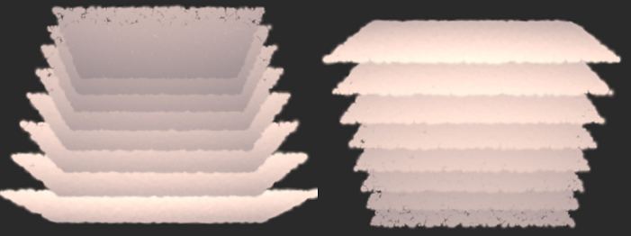
After going through the trouble of computing the shadow for each particle, we need to render them in the correct order. This is important because in alpha blending a + b does not equal b + a. For example, if a darkened particle is behind a lit particle, but rendered on top, the result will be darker than expected. You can see this happen in the image below. On the right, the particles are renderered in correct order, while on the left they are renderered in the wrong order.

So we need a way of sorting the particles each frame, fast. And it would be best if we could do this on the GPU, as transferring data back and forth to the CPU is way too slow. Various sorting algorithms have been designed to run well on GPUs, taking advantage of parallelism and cache locality. In our sample we use a well known parallel radix sort ([8], [9], [10]). I'll explain how it works with an example.

The main idea of the sorting algorithm is based on counting. For example, say that we need to put the number 3 in a set ordered by increasing value. If we know that there are in total 5 numbers less that 3 in our input, then we know that 3 must come after all of these - that is, in position 5.

To determine such a count for each number in our input, we use a prefix sum (also known as a scan). The prefix sum of a sequence is a new sequence, where each element is the sum of elements before it. It is either inclusive or exclusive, depending on whether the current element is included or not. For example:

Input:     1  2  3  4  5
Exclusive: 0  1  3  6 10
Inclusive: 1  3  6 10 15        

Note that the final element of the inclusive scan is the sum of all the inputs. Now let's consider a series of 2-bit numbers as our input that we wish to sort. For each possible digit, we need to count the number of numbers less than it, that have appeared earlier in the sequence. To do this we construct four flag arrays, one for each possible digit, that have a 1 where the number in the input matches the digit, and 0 elsewhere:

Input:  1 3 2 0 1 0 2 2
Flag 0: 0 0 0 1 0 1 0 0
Flag 1: 1 0 0 0 1 0 0 0
Flag 2: 0 0 1 0 0 0 1 1
Flag 3: 0 1 0 0 0 0 0 0

If we do an exclusive prefix sum over the flags, and carry over the total sum from each array to the next, we get:

Scan 0: 0 0 0 0 1 1 2 2 
Scan 1: 2 3 3 3 3 4 4 4 
Scan 2: 4 4 4 5 5 5 5 6 
Scan 3: 7 7 8 8 8 8 8 8  (Note that 7 was carried over instead of 6)

And this table tells us all we need to shuffle the input in the correct order!

If we look at the first column of the flag arrays, we see that digit 1 is flagged. This means that we should look in the row for digit 1 of the scan table above to find the new location for the element. We do so, and find the offset to be 2. Thus, in the sorted array, the first 1 should be placed at index 2. Verifying that this is indeed correct is left as an exercise to the reader.

The final radix sort algorithm works by sorting two and two bits of the input values using the above method, starting from the least significant digit and moving to the most significant digit. We could use other n-bit radices, but we found that a 2-bit radix gave nice performance. Furthermore, a nice trick we can do with 2-bit radices is to pack the elements of the flag and scan arrays into vec4s, allowing us to handle all arrays simultaneously using vector operations.

For efficiency, this demo implements the radix sort as four different compute shader programs. The prefix sum is calculated in blocks in scan.cs and scan_first.cs (first pass shader). The individual blocks are then merged into a single prefix sum in scan_resolve.cs and scan_reorder.cs. See the code for more technical details.

The Application

The application consists of a single particle emitter flying around in the scene. A green sphere can be moved around by dragging along the floor, and the camera can be rotated by dragging along the sky. In the code there are various parameters that can be adjusted, such as the particle radius, smoke color and light position.