 |
OpenGL ES SDK for Android
ARM Developer Center
|
|
OpenGL ES SDK for Android
ARM Developer Center
|
This sample will show you how to efficiently implement high quality ocean water rendering using compute shaders in OpenGL ES 3.1.
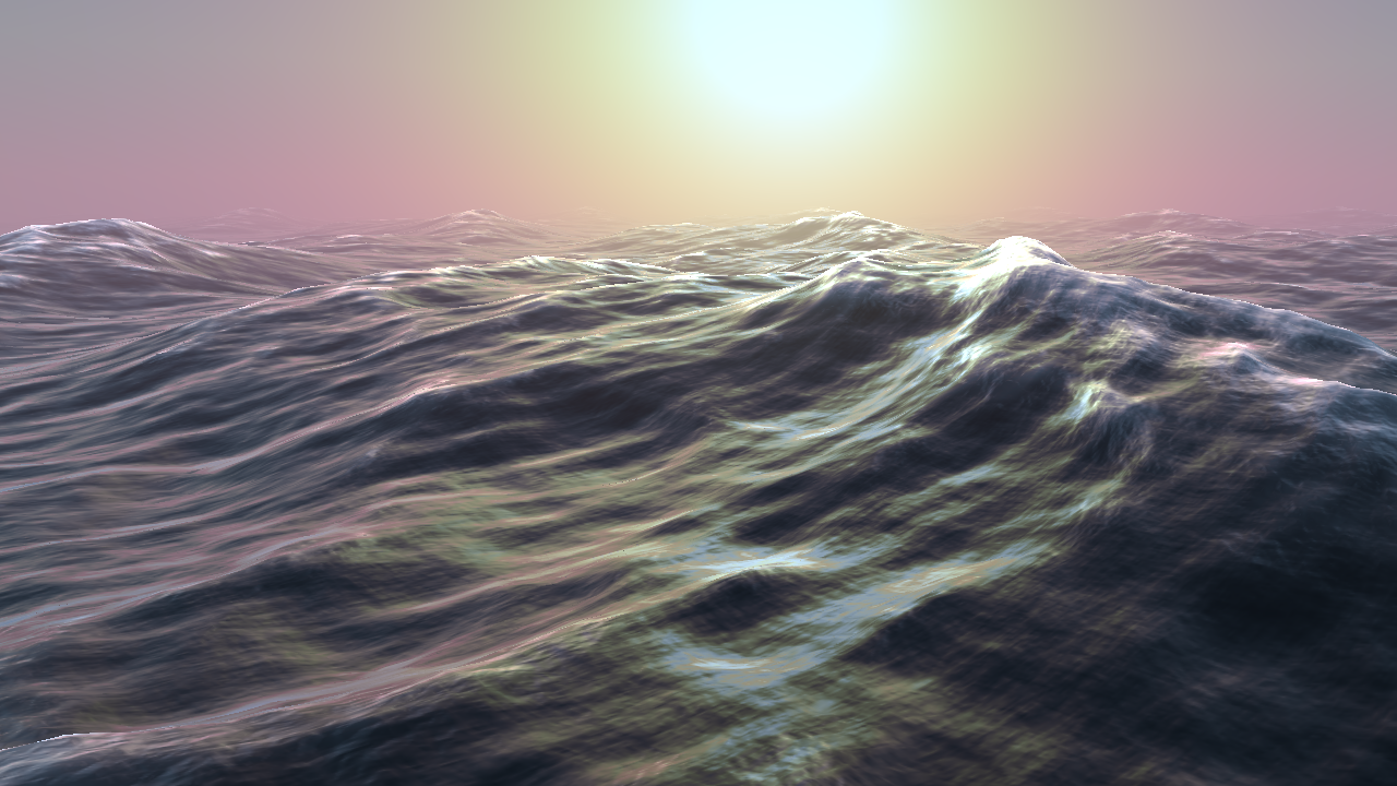
The ocean rendering technique in this sample is based on the well-known water rendering paper by J. Tessendorf [1] which implements heightmap generation by synthesizing a very large number of waves using the Fast Fourier Transform.
The main principle of Ocean rendering is that it can be modelled very well by thinking of it a sum of "infinite" waves at different amplitudes travelling in different directions.
Summing up a large number of sinusoids is very intensive with a naive approach, and has complexity O(M * N) if synthesizing M waves into N samples in one dimension. Increasing this to two dimensions and we end up with a terrible O(M * N^2) complexity. With simpler water techniques, very few waves are therefore used instead and the sinusoids are accumulated directly. For realistic looking water, we would really prefer the number of waves to be the same as number of samples.
The inverse fast Fourier transform does this excellently, using only O(2N * (N * log2(N))) complexity for a 2D NxN grid to synthesize NxN waves. For reasonable values (this sample uses N = 256), this can be done very efficiently on GPUs.
There are many excellent introductions to the Fast Fourier Transforms, so only a short introduction will be provided here. The core of the Fourier Transform is a transform which converts from the time/spatial domain to frequency domain and back. The mathematical formulation of the discrete (forward) Fourier Transform is:
and inverse Fourier Transform which we're mostly interested in here:
j is the imaginary constant sqrt(-1) which is also knows as "i". Thus, the Fourier Transform is formulated with complex numbers. Taking the exponential of an imaginary number might look weird at first, but it can be shown using Taylor expansion that exp(j * x) is equivalent to
If we imagine that the real and imaginary numbers form a 2D plane, exp(j * x) looks very much like rotation with angle x. In fact, we can simply think of exp(j * x) as a complex oscillator.
This is the core of ocean wave synthesis. In the frequency domain, we will create waves with certain amplitudes and phases, and use the inverse Fourier transform to generate a sum of sinusoids. To move the water, we simply need to modify the phases in the frequency domain and do the inverse FFT over again.
Since the FFT assumes repeating inputs, the heightmap will be tiled with GL_REPEAT wrapping mode. As long as the heightmap is large enough, the tiling effect should not be particularly noticable.
The GPU FFT implementation used in this sample is based on the GLFFT library [2]. The FFT implementation in GLFFT is inspired by work from E. Bainville [3] which contain more details on how FFT can be implemented efficiently on GPUs.
The ocean is a random process in that the amplitudes and phases of waves are quite random, however, their statistical distributions are greatly affected by wind and can be modelled quite well. The Tessendorf paper [1] uses the Phillips spectrum which gives the estimated variance for waves at certain wavelengths based on wind direction and speed.
Based on this formula, we generate a random two-dimensional buffer with initial phase and amplitude data for the heightmap and upload this to the GPU only at startup.
In Fourier Transforms, we need to consider negative and positive frequencies. Before computing the spatial frequency, we alias the frequency according to Nyquist. This means that the higher values for x and z will alias to the negative frequencies. The negative frequencies represent waves travelling in the opposite direction as the positive counterparts.
Before actually doing the FFT on the GPU, we run compute shader passes which generates a new frequency domain buffer for height, normals and displacement.
While the frequency space is indeed complex, the final heightmaps we're interested in contain real data. Since the frequency samples generated by generate_heightmap() are complex conjugated, we can use a clever two-for-one FFT scheme which can do complex-to-real FFT at close to 2x improvement in both speed and power.
For the normal map and displacement map however, we need two components, so we do a regular complex-to-complex FFT in this case.
After generating the iFFTs, we generate heightmap normals, compute the Jacobian, and various other things, before mipmapping the textures.
Using a FP16 FFT instead of FP32 FFT works well in this sample and this saves lots of extra bandwidth and computation in the FFT implementation.
One important detail with mipmapping the heightmap is that we cannot use a box filter. Instead, we pretend that the first texel lies on uv = (0, 0). This is necessary later when we want to properly render the heightmap. It is also necessary to mipmap our heightmap with compute shaders. The alternative is to compute the mipmap with fragment shaders, but for a tiled architecture such as Mali, having vertex shading (which uses the heightmap) depends on fragment (mip-generation) often creates a bad pipeline stall.
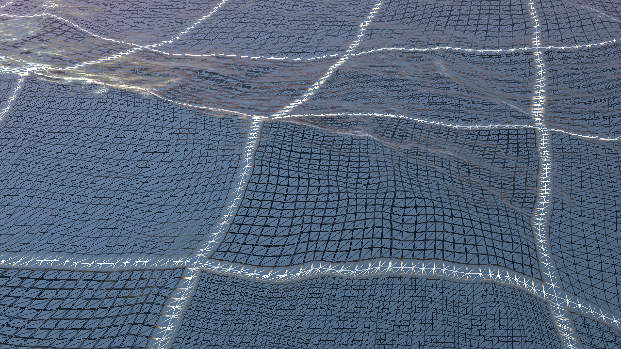
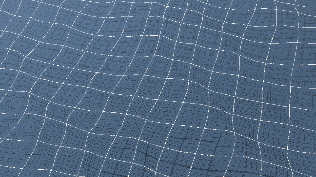
In reality, ocean waves do not behave like pure sinusoids, but behave in a more "choppy" way where peaks of the waves compact a bit, to make the waves look sharper.
Using only a straight heightmap, this is not easy to implement, however, we can have another "displacement" map which computes displacement in the horizontal plane as well. If we compute the inverse Fourier transform of the gradient of the heightmap, we can find a horizontal displacement vector which we will push vertices toward. This gives a great choppy look to the waves.
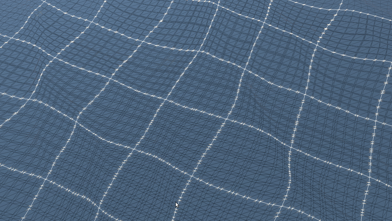
By adding choppiness, we can go from
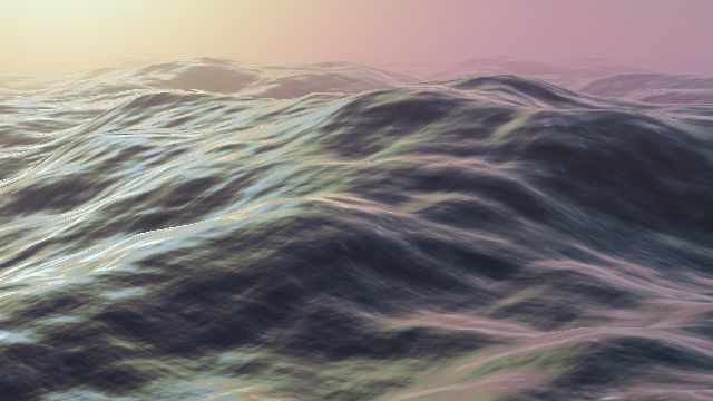
to
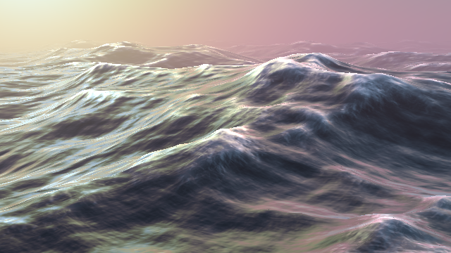
We implement it in compute shaders by modifiying generate_heightmap() slightly.
See [1] for mathematical details.
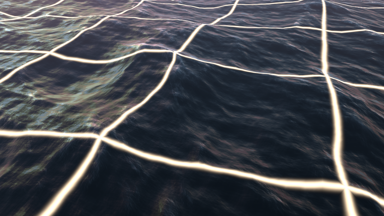
At wave crests, the turbulence tends to cause a more diffuse reflection, increasing overall brightness and "whiteness" of the water. By looking at the gradient of the horizontal displacement map, we can detect where the crests occur and use this to pass a turbulence factor to the fragment shader.
When the Jacobian factor is close to 0, the water is very "turbulent" and when larger than 1, the water mesh has been "stretched" out. A Jacobian of 1 is the "normal" state.
We combine the lower-frequency Jacobian with the normal map in the fragment shader to compute a final "turbulence" factor which creates a neat shading effect.
Rendering heightmaps (terrains) efficiently is a big topic on its own. For this sample, we implement two different approaches to rendering continous LOD heightmaps. Both variants have a concept of patches which are adaptively subdivided based on distance to camera.
First we place a large grid of patches in the world. The patches are roughly centered around the camera, but they do not move in lock-step with the camera, rather, they only move in units of whole patches in order to avoid the "vertex swimming" artifact.
With this scheme, we want to subdivide the patches depending to distance to camera. The full grid is quite large, so we cannot have full quality for the entire world without taking a serious performance hit.
We also want a "continous" LOD effect. A difficult problem to solve is avoiding "popping" artifacts and "swimming" artifacts at the same time. Popping happens when the vertex mesh suddenly changes resolution without any kind of transition band. Vertex swimming happens if we move the heightmap (and hence texture sampling coordinates) around without snapping it to some kind of grid.
For adaptively subdividing a patch, Tessellation in OpenGL ES 3.2 [7] can solve this quite neatly.
We implement tessellation by treating our water patch as a GL_PATCH primitive. In the control shader, we compute tessellation factors for our patch.
For the outer tessellation factors, it is vital that the tessellation factors are exactly the same for patches which share edges, otherwise, we risk cracks in the water mesh, which is never a good sign.
To make this work, we find tessellation factors in the four corners of our patch. We then take the minimum LOD of two corners which belong to an edge, which decides the tessellation factor for that edge.
In order to avoid processing patches which are outside the camera, we frustum cull in the control shader as well, and set tessellation factors to negative values which discards the patch outright.
In the evaluation shader, we interpolate the corner LODs calculated by the control shader to figure out which LOD we should sample the heightmap with.
When sampling the heightmap, we need to take extra care to make sure we avoid the swimming artifact. A simple and effective way to make sure this happens is that when we sample the heightmap, we sample the respective mipmaps between their texels so the bilinear interpolation is smooth and has a continuous first derivative. For this reason, we cannot use tri-linear filtering directly, but we can easily do this ourselves. Ideally, we would like uv = (0, 0) to land exactly on the first texel here since that would also map to first texel in the next miplevel, however, this is not the case with OpenGL ES. For this, reason, we apply the half-texel offsets independently for every level. The speed hit here is negligible, since tri-linear filtering generally does two texture lookups anyways.
The second thing we need to take care of is using the appropriate subdivision type. Tessellation supports equal_spacing, fractional_even and fractional_odd. We opt for fractional_even here since it will interpolate towards an even number of edges which matches well with the textures we sample from. We want our vertex grid to match with the texel centers on the heightmap as much as possible.
For devices which do not support tessellation, we implement a heightmap rendering scheme which takes inspiration from tessellation, geomipmaping [4], geomorphing [5] and CDLOD techniques [6], using vertex shaders and instancing only.
Like geomipmapping and geomorphing, the patch size is fixed, and we achieve LOD by subdividing the patch with different pre-made meshes. Like CDLOD, we transition between LODs by "morphing" the vertices so that before switching LOD, we warp the odd vertices towards the even ones so that the fully warped mesh is the same as the lower-detail mesh, which guarantees no popping artifacts. Morphing between LODs and using a fixed size patch is essentially what tessellation does, so this scheme can be seen as a subset of quad patch tessellation.
One of the main advantages of this scheme over CDLOD is its ability to use a different LOD function than pure distance since CDLOD uses a strict quad-tree structure purely based on distance. It is also simpler to implement as there is no tree structure which needs to be traversed. There is also no requirement for the patches to differ by only one LOD level as is the case with CDLOD, so it is possible to adjust the LOD where the heightmap is very detailed, and reduce vertex count for patches which are almost completely flat. This is a trivial "LOD bias" when processing the patches.
The main downsides of this algorithm however is that more patches are needed to be processed individually on CPU since there is no natural quad-tree structure (although it is possible to accelerate it with compute and indirect drawing) and for planetary style terrain with massive differences in zoom (e.g. from outside the atmosphere all the way into individual rocks), having a fixed patch size is not feasible.
To allow arbitrary LOD between patches, we need to know the LOD at all the four edges of the patch and the inner LOD before warping our vertex position. This info is put in a per-instance uniform buffer.
We also want to sample our heightmap using a LOD level that closely matches the patch LOD. For this, we have a tiny GL_R8 LOD texture which has one texel per patch and we can linearly interpolate the LOD factors from there. We update this texture when processing the patches.
Building the UBO is also quite simple. To select LODs we look at the four neighbor patches. The edge LOD is the maximum of the two neighbors. We need the maximum since otherwise there would not be enough vertices in one of the patches to correctly stitch together the edge.
While we could in theory use the LOD factor we generate in warp_position() to sample the heightmap, this would break the corner vertices on the patch. We need to make sure all vertices that are shared between patches compute the exact same vertex position. This is not the case with the vlod factor we compute in warp_position().
From here, we sample our heightmaps, etc as before, very similar to the evaluation shader implementation.
While correctly shading ocean water is a big topic entirely on its own, this sample uses a simple approach of cubemap reflection against a pregenerated skydome. For more realistic specular shading, the fresnel factor is added in. No actual diffuse shading is used, and the only source of lighting is the skydome cube map.
The shader samples two normal (gradient) maps, one low-resolution map generated from the heightmap, and one high-frequency gradient map which is also generated using FFT.
[1] J. Tessendorf - Simulating Ocean Water - http://graphics.ucsd.edu/courses/rendering/2005/jdewall/tessendorf.pdf
[2] GLFFT - Fast Fourier Transform library for OpenGL - https://github.com/Themaister/GLFFT
[3] E. Bainville - OpenCL Fast Fourier Transform - http://www.bealto.com/gpu-fft.html
[4] W. H. de Boer - Fast Terrain Rendering Using Geometrical MipMapping - http://www.flipcode.com/archives/article_geomipmaps.pdf
[5] D. Wagner - Terrain Geomorphing in the Vertex Shader - https://www.ims.tuwien.ac.at/publications/tuw-138077.pdf
[6] F. Strugar - Continous Distance-Dependent Level of Detail for Rendering Heightmaps (CDLOD) - http://www.vertexasylum.com/downloads/cdlod/cdlod_latest.pdf
[7] GL_EXT_tessellation_shader (now OpenGL ES 3.2) - https://www.khronos.org/registry/gles/extensions/EXT/EXT_tessellation_shader.txt

